
Let’s talk about reward and value
Published:
I will skip the notation and introduction on RL as a Markov Decision Process, for that you can refer to this blog. Here is a checklist of questions to ask yourself before proceeding:
- what $J(\theta)$ and $\nabla_{\theta} J(\theta)$ (recall policy gradient theorem) look like?
- what is $Q$, $A$, $V$?
- do you have 10 minutes to spare?
Let’s recall the REINFORCE algorithm which has a gradient form of: \(\nabla_{\theta} J(\theta) = \mathbb{E}_{\pi}[Q(s,a)\nabla_{\theta} \log \pi(a \mid s)]\)
since $Q(s_t,a_t) = \mathbb{E}_{\pi}[G_t \mid s_t, a_t]$, we have: \(\nabla_{\theta} J(\theta) = \mathbb{E}_{\pi}[G_t \nabla_{\theta} \log \pi(a_t \mid s_t)]\)
recall the $G_t$ is the discounted return, essentially a function that takes a trajectory and returns a scalar. This allows us to estimate $G_t$ in a Monte Carlo way, thus estimating the poliy gradient in a Monte Carlo way.
Usually a baseline $b(s)$ is subtracted from $Q(s,a)$ to reduce the variance of the gradient estimate. The ideal candidate is the value function $V(s)$, but in practice, we have some expected future cumulative reward from the episodes/rollouts, which is $\frac{1}{N} \sum_{i=1}^{N} G_i$ for $N$ rollouts, then one would fit a value network to minimize the loss:
\[L(\theta) = \frac{1}{\sum_{i} T_i}\sum_{i=1}^{N} \sum_{t=1}^{T} ( G_{i,t} - V_{\phi}(s_{i,t}))^2\]Given a trajectory i, the estimated advantage $A_{i, t} = G_{i, t} - V_{\phi}(s_{i, t})$ replaces the $Q(s,a)$ in the REINFORCE sample-based gradient formula.
note: the baseline can be any function of the state, not necessarily the (estimated) value function, but the variance is minimized when the baseline is the value function.
This snippet from the seminal GAE paper summarizes the usual forms of policy gradient. 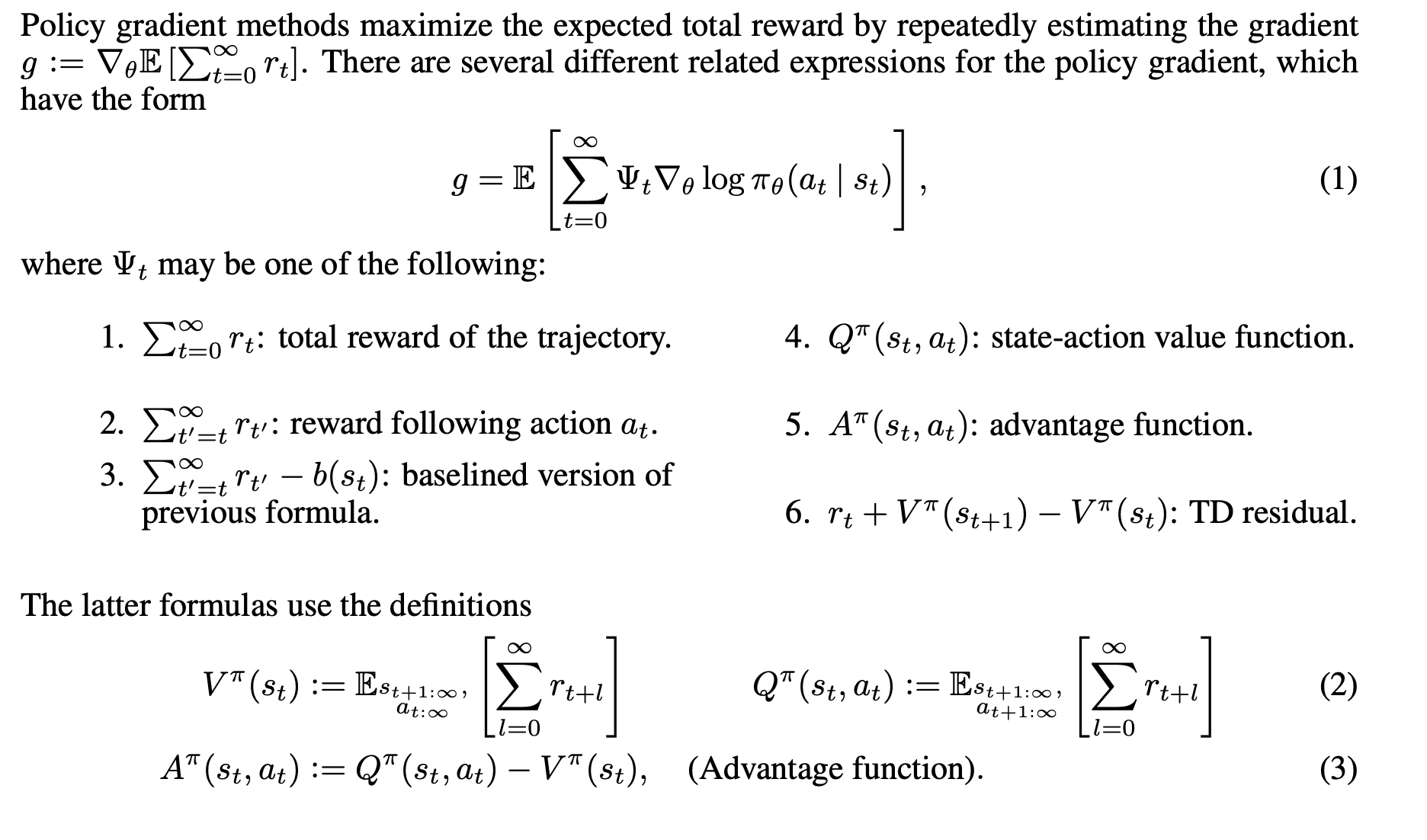
- item 1 and 2 correspond to the vanilla sample-based REINFORCE.
- (Monte Carlo) item 3 corresponds to the variance reduced REINFORCE.
- item 4 corresponds to the canonical form of policy gradient theorem.
- item 5 is the expectation of item 3, over all possible trajectories.
- (Bootstrapping) item 6 is the TD estimate of the advantage function.
using the adavantage function is theoretically golden as it minimizes the variance of the gradient estimate. So our obvious philosophy is reduce the problem of estimating policy gradient to the problem of estimating adavantage function.
Note: the freedom of choosing the baseline gives birth to many algorithms that don’t train a separate value network, but using some sort of statistics from all rollouts as the baseline, such as GRPO.
This is where Monte Carlo and Bootstrapping come into play.
Monte Carlo
$\sum_{t’ = t} r_{t’} - V_{\phi}(s_t)$ can be golden as well because it is unbiased and low variance (if the value estimation is good). But it can still work with a random value network when the number of episodes is large enough.
Bootstrapping
the formula $r_t + \gamma V_{\phi}(s_{t+1}) - V_{\phi}(s_t)$ may look ugly, but here is the interpretation: both $r_t + \gamma V_{\phi}(s_{t+1})$ and $V_{\phi}(s_t)$ are adavantage estimates, but since $r_t + \gamma V_{\phi}(s_{t+1})$ contains a real step, it is more accurate than $V_{\phi}(s_t)$. Thus we nudge the value network to minimize the error over all episodes and steps.
Generalized Advantage Estimation (GAE) essentially creates a slider between the two approaches using a hyperparameter called $\lambda$ (lambda).
It recognizes that Item 3 (Monte Carlo) and Item 6 (TD Error) are just two extremes of a spectrum involving bias and variance. GAE allows you to pick a “sweet spot” in the middle.
GAE starts by calculating the TD error (Item 6) for every single step in the trajectory. Let’s call this $\delta_t$:
\[\delta_t = r_t + \gamma V(s_{t+1}) - V(s_t)\]GAE defines the advantage as an exponentially weighted sum of these TD errors into the future.
\[\hat{A}_t^{GAE} = \sum_{l=0}^{\infty} (\gamma \lambda)^l \delta_{t+l}\] \[= \delta_t + (\gamma \lambda)\delta_{t+1} + (\gamma \lambda)^2\delta_{t+2} + \dots\]Here is how varying $\lambda$ (from 0 to 1) allows GAE to interpolate perfectly between your two items:
Scenario A: $\lambda = 0$ (Pure Item 6)
If you set $\lambda = 0$, the decay is instant. The sum cuts off after the first term.
\[\hat{A}_t = \delta_t = r_t + \gamma V(s_{t+1}) - V(s_t)\]Scenario B: $\lambda = 1$ (Pure Item 3)
If you set $\lambda = 1$, the sum includes all future TD errors. Something mathematical magic happens here called a “telescoping sum.” The intermediate Value terms cancel each other out: \(\hat{A}_t = (r_t + \gamma V_{t+1} - V_t) + \gamma(r_{t+1} + \gamma V_{t+2} - V_{t+1}) + \dots\)
- The $+ \gamma V_{t+1}$ from the first term cancels with the $-\gamma V_{t+1}$ from the second term.
- Eventually, you are left with only the raw rewards and the initial baseline: \(\hat{A}_t = \left( \sum_{k=0}^\infty \gamma^k r_{t+k} \right) - V(s_t) = G_t - V(s_t)\)
Actor-Critic Algorithms
Now we can talk about Actor-Critic algorithms, not all algorithms mentioned below are REINFORCE-type algorithms, because some are value-based algorithms.
So you can:
- plug in either $Q$ or $A$ into the REINFORCE formula, means you need to estimate either state-action value or state value.
- update the policy using REINFORCE once we estimated $Q$ or $A$, this is policy-based, but you can also deterministically choose the action based on $Q$ or $A$, this is value-based.
- you can choose between on-policy and off-policy learning.
$2^3 = 8$. Let’s list 8 canonical algorithms in each category.
| Strategy | Data | Target: Q-Function ($Q_w$) | Target: V-Function ($V_w$) |
|---|---|---|---|
| Value-Based | Off-Policy | 1. DQN The classic Q-learning. Learns the optimal $Q^*$, acts greedily. | (Requires Model) Cannot act model-free. |
| Value-Based | On-Policy | 2. SARSA Updates $Q^\pi$ using the actual action taken ($s, a, r, s’, a’$). | (Requires Model) Cannot act model-free. |
| Policy-Based | Off-Policy | 3. DDPG / SAC Learns $Q(s,a)$ to tell the actor which continuous action is best. | 4. IMPALA / V-trace Learns $V(s)$ and uses importance sampling corrections to estimate advantages off-policy. |
| Policy-Based | On-Policy | 5. Vanilla Actor-Critic $\nabla \ln \pi \cdot Q_w$. theoretically inferior to PPO. | 6. PPO / A2C The standard policy-based one, used with GAE. |
It is really important to understand PPO, so I took this pseudo-code from here to explain the PPO algorithm. 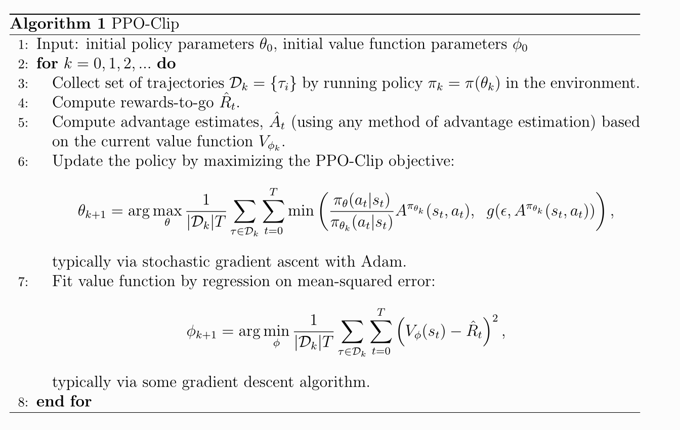
the “any method of advantage estimation” is usually GAE.
So far we have neglected the rewards, where do they come from? Do we have access to a scalar after each action? Do we even have access to any reward signal at all in reality?
In aligning pretrained LLMs, unfortuantely, neither step-wise reward nor episode-wise reward is available, because human annotation is not available for all rollouts.
Thus a reward model is trained to provide a scalar reward after each action, or a scalar reward after each episode. Then… we can use PPO… except that training all these models together is highly unstable so we use DPO… anyways, let’s skip RLHF, and talk about reasoning where preference optimization cannot be used.
to build a long-horizon reasoning agent, we are faced with a new set of problems: given verifiable reward, a scalar per episode:
- how to assign action-level rewards? Especially when the trajectory is very long? This is called credit assignment, sometimes called process reward in LLM literature.
- what is the granularity of action? This is fundamental, can be token-as-an-action or tool-call-as-an-action, like in multi-turn RL.
- do we need a value model? How do we fit a value model?
Merry Christmas!
update: Jan 15, 2026
Happy new year! I have been busy with another that actually uses RL heavily so I will come back to share more on both the theory and some lessons I learned from the practical/engineering side of the project.