Single-Rollout Agent RL: SAO, FlashREINFORCE, BPO and KLPO
Published:
In this post we study recent algorithmic progress on two fundamental RL questions: credit assignment on the theory side, and asynchronous inference-trainer separation on the practical side. GRPO, SAO, FlashREINFORCE, BPO and KLPO each answer that pair differently.
1. Setup: why single-rollout agent RL?
For a prompt \(x\), GRPO-like methods sample several complete responses from the same prompt and use their rewards to form a prompt-specific baseline. If the rewards are \(R_1,\ldots,R_G\), a basic group-centered signal is:
The main appeal is that it is simple and critic-free: the group mean is a drop-in baseline, so no value network has to be trained, and value networks are hard to fit for long, sparsely rewarded trajectories. It also controls for task difficulty as a side effect, since the baseline is computed per prompt. But long-running agents make groups operationally expensive:
- one training prompt consumes \(G\) complete agent attempts;
- a group cannot be finalized until slow siblings finish. This is the straggler problem, and the synchronization barrier it imposes is a major source of slowdown in RL training;
- during those minutes, the learner may already have moved several policy versions ahead. This demands a correction for the sampling distribution, which we come back to throughout the post, and it is a known source of instability: naive off-policy training on stale data degrades or collapses. M2PO (2025) traces much of that collapse to over-aggressive clipping of high-importance-weight tokens rather than to staleness itself, and shows that stale data can match on-policy data when the correction is handled carefully, but the failure mode is real either way.
SAO
Keep PPO's actor-critic machinery. Replace the group baseline with a learned value function.
FlashREINFORCE
Remove both the group and the critic. Use batch-centered terminal reward plus explicit stale-policy controls.
2. SAO: PPO adapted to single-rollout asynchronous agents
The most useful shorthand is: SAO is essentially actor-critic PPO in the single-rollout asynchronous-agent regime.
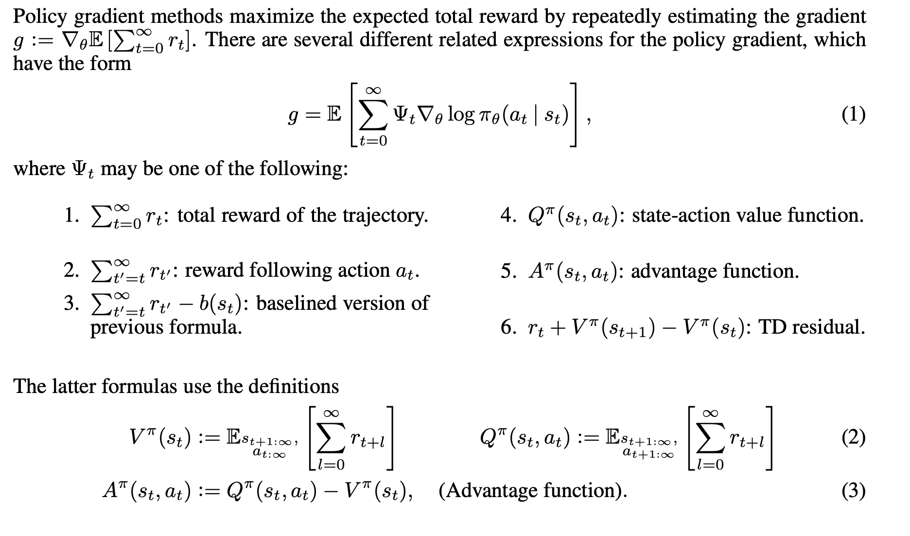
Because it inherits that machinery wholesale, let's review the common objects from PPO first: the critic, the TD residual, and GAE. Only then do we look at what SAO changes.
2.1 Critic, TD residual, and GAE
The actor is \(\pi(a\mid s)\). The critic estimates expected future return \(V(s)\). A one-step TD residual is:
With terminal-only rewards, most intermediate \(r_t=0\). GAE aggregates future TD residuals:
A worked example on one trace
Take a four-step trace with a terminal reward only, and set \(\gamma=1\), \(\lambda=0.5\). The agent succeeds, so \(r_4=R=1\) and \(r_1=r_2=r_3=0\). Suppose the critic reports the values in the second column. Everything else follows from the two formulas above.
| \(t\) | \(V(s_t)\) | \(r_t\) | \(\delta_t=r_t+V(s_{t+1})-V(s_t)\) | \(A_t=\delta_t+0.5\,A_{t+1}\) |
|---|---|---|---|---|
| 1 | 0.5 | 0 | \(0+0.6-0.5=0.1\) | \(0.1+0.5(0.05)=\mathbf{0.125}\) |
| 2 | 0.6 | 0 | \(0+0.4-0.6=-0.2\) | \(-0.2+0.5(0.5)=\mathbf{0.05}\) |
| 3 | 0.4 | 0 | \(0+0.8-0.4=0.4\) | \(0.4+0.5(0.2)=\mathbf{0.5}\) |
| 4 | 0.8 | 1 | \(1+0-0.8=0.2\) | \(0.2+0.5(0)=\mathbf{0.2}\) |
| 5 | 0 (terminal) | n/a | n/a | \(A_5=0\) |
Read the last column bottom-up: the recursion starts from \(A_5=0\) and walks backward, which is why each row needs the row below it.
Two things are worth noticing. First, one scalar reward at the end produced four different advantages, ranging from \(0.05\) to \(0.5\). Step 3 is credited ten times as strongly as step 2, because the critic says the state improved sharply there \((0.4\to0.8)\) while step 2 looked like a step backward \((0.6\to0.4)\). Second, \(\delta_2\) is negative even though the trace succeeded: the critic thought that move made things worse, and GAE only rescues it to a slightly positive \(A_2\) because the later steps went well.
As a sanity check, \(\lambda=1\) makes the recursion telescope back to \(A_t=R-V(s_t)\). Here that gives \(A_1=0.1-0.2+0.4+0.2=0.5=1-V(s_1)\). So \(\lambda\) interpolates between trusting the critic step by step \((\lambda=0)\) and ignoring it in favor of the realized return \((\lambda=1)\).
This per-token resolution is what the critic buys, and it is the main thing the critic-free methods later in this post give up.
2.2 Skip-observation GAE
An agent trajectory alternates between model-controlled actions and externally generated observations:
MODEL:        run pytest
ENVIRONMENT:  stack trace, file contents, tool output ...
MODEL:        edit auth.py
Write \(a_{i,N}\) for the last token of action \(i\), \(o_i\) for the observation block the environment returns, and \(a_{i+1,0}\) for the first token of the next action. Ordinary token-level GAE takes the value difference between adjacent tokens, so at this boundary it would compute:
SAO instead modifies the Bellman target to bypass the environment tokens and link the value of the current action directly to the value of the next one:
The entire difference is one term: \(V(o_{i,\text{start}})\) becomes \(V(a_{i+1,0})\). The recursion then chains action to action, and every token inside an action inherits its advantage from that chain. The paper's motivation is that the transition from the end of an action into an observation is discontinuous from the model's perspective, since the model did not generate \(o_i\); bridging the gap keeps the stochasticity of environment feedback out of the advantage estimate.
How well is this component isolated?
The paper never ablates skip-observation GAE on its own. Its ablation tables vary the value-model training strategy, the critic update frequency, and the importance-sampling scheme, but no row turns the observation-bypassing Bellman target off and runs with plain token-level GAE through the observation. So the design is argued for, not measured in isolation.
The nearest experimental evidence is the granularity ablation (Table 5 and Figure 6 in the paper), which asks a related question: at what resolution should credit be assigned inside an agent step?
| Credit granularity | AIME2025 | BeyondAIME |
|---|---|---|
| Step-level (average over the action) | 85.8 | 60.5 |
| Step-level (last token of the action) | 87.3 | 62.8 |
| Token-level | 89.8 | 66.8 |
2.3 Training the value model
The critic is the fragile part of the design, and SAO spends a lot to keep it steady. The loss itself is ordinary regression onto the realized return, \(\mathcal L^{\mathrm{VF}}_\phi=\mathbb E\bigl[(V_\phi(q,y_{\lt t})-R)^2\bigr]\); the choices around it are what matter. During RL the attention modules of \(V_\phi\) are frozen and only the MoE projections train, worth about 7 points on AIME2025. The critic takes \(K=2\) updates per policy step rather than one, worth another 2 points on AIME2025 and 5 on BeyondAIME. GAE is length-adaptive, \(\lambda_{\text{policy}}=1-1/(\alpha l)\) with \(\alpha=1.5\), so the effective horizon scales with trajectory length \(l\). And a 10-step warmup plus a scaled-up value pretraining corpus answers the cold-start problem, since a fresh critic emits noise and single-rollout training has no group baseline to fall back on while it settles. On that last point the paper is silent about provenance: it says only that it significantly increased the scale of the value pretraining corpus, never what that corpus is or which policy generated it, so this is the one part of the recipe a reader cannot reproduce from the paper alone.
2.4 One asynchronous batch of eight prompts
| Prompt | Rollout policy | Length | Reward |
|---|---|---|---|
| x1 | v100 | 800 | 1 |
| x2 | v100 | 1400 | 0 |
| x3 | v101 | 600 | 1 |
| x4 | v101 | 2200 | 0 |
| x5 | v102 | 900 | 1 |
| x6 | v102 | 1100 | 0 |
| x7 | v103 | 750 | 1 |
| x8 | v103 | 3000 | 0 |
Suppose the learner is now at v105. Each rollout stored the probability under the behavior policy \(\mu\), while the learner recomputes the current probability under \(\pi\).
2.5 Why token importance correction is \(\pi/\mu\)
It is ordinary change of measure. For any quantity \(f(a)\):
Conditioned on a stored history \(h_t\), SAO therefore uses:
SAO then applies a direct double-sided mask, which the paper calls Direct double-sided Importance Sampling (DIS). The trust region is the interval \([1-\epsilon_\ell,\,1+\epsilon_h]\) and the calibration function zeroes everything outside it:
So a token whose ratio strays too far from one is removed from the policy gradient entirely, rather than merely PPO-clipped to the boundary. Note that the bounds are asymmetric and quite wide in practice: \(\epsilon_\ell=0.3,\ \epsilon_h=5.0\) for math reasoning with Python, and \(\epsilon_\ell=0.8,\ \epsilon_h=3.0\) for coding.
The subtle limitation is that \(\rho_t\) corrects the sampled action given the stored history. The history itself was generated by \(\mu\). Exact trajectory importance correction would involve a product of prefix ratios, which is generally unusably high-variance for long LLM trajectories.
3. FlashREINFORCE: critic-free single-rollout RL
Flash keeps the one-rollout asynchronous setting but removes \(V(s)\), TD errors, and GAE. The whole method fits in three pieces:
1. One-batch update with mean baseline
Center one fresh batch, update once, discard. No group wait and no replay.
2. Sequence trust region
Accept the trajectory only if the mean sampled-action proxy is at or below the sequence threshold.
3. Sample-mean loss instead of token-mean loss
\(A_i\): centered advantage. \(\pi_\theta/\mu_i\): learner-to-behavior ratio. \(T_i^{-1}\): within-trajectory average. \(m_i\): one admission decision for the complete trajectory.
FlashREINFORCE at a glance. Each fresh batch supplies its own baseline, receives one update, and is discarded. Sequence trust screens complete trajectories; the sample mean limits length-amplified negative updates.
3.1 One-Batch REINFORCE
For a batch of independently completed trajectories, Flash uses a trajectory-level centered reward:
All policy tokens in one trajectory receive this same basic scalar advantage. This is much coarser credit assignment than SAO.
3.2 Token-level importance correction
Stale trajectories are still collected under an older behavior policy \(\mu_i\), so Flash uses the same local change-of-measure ratio:
Again, this corrects the action distribution conditional on a stored history, not the probability of reaching that history.
3.3 Sequence Trust Region
This is the same gap we hit in the SAO section: the ratio corrects the sampled action given the prefix, but the prefix itself is already stale. Flash does not try to correct for that. Instead it adds a gate, a trajectory-level staleness test, and that test is worth unpacking. At each sampled token, let:
Collapse the vocabulary into two events, \(\{a_t,\text{everything else}\}\), and compute the Bernoulli KL:
The Flash paper credits this proxy to DPPO (Qi et al., 2026). We will meet the same computational trick, collapsing the vocabulary to two events, again in BPO, where it falls out of a different derivation entirely.
The trajectory drift statistic is the mean:
The whole trajectory is admitted only if \(\bar D_i\) is below the trust threshold.
Why a sum of token divergences is natural
Autoregressive trajectory probabilities factorize, so log likelihood ratios and trajectory KL decompose additively across conditional token distributions. Flash then divides by \(T_i\) so the threshold measures average per-token staleness rather than automatically rejecting longer trajectories. Note that this runs contrary to Dr.GRPO and sits much closer to the original GRPO, which uses a sample-level normalization that actually makes the estimator biased.
Why Bernoulli KL?
Storing the full old-policy vocabulary distribution at every prefix is expensive. The Bernoulli coarsening needs only the sampled-token probability. By data processing, this coarsened KL is no larger than the full categorical KL, so it is a cheap proxy, not a certificate that the full distributions are close.
3.4 Sample-Mean Optimization and the Dr.GRPO tension
Flash first averages within each trajectory:
This gives each trajectory roughly equal outer weight, so one 10k-token failed wander does not automatically contribute twenty times the gradient mass of a 500-token failure.
Flash directly ablates this against token-mean aggregation and reports materially worse long-horizon behavior when removing the per-trajectory normalization. The Flash paper does not discuss Dr.GRPO, but the comparison is worth drawing: this is not the Dr.GRPO correction but its mirror image. Dr.GRPO argues that realized \(1/T_i\) normalization changes the episodic policy-gradient objective and can under-penalize long incorrect responses, and Flash accepts that reweighting anyway because it empirically stabilizes long agent rollouts.
For the sequence-level gate, the Flash paper cites Trust Region Masking for Long-Horizon LLM Reinforcement Learning alongside Seq-MIS as motivation for sequence-level admission. TRM makes the same argument that local token-ratio control does not by itself control accumulated long-horizon distribution shift.
4. SAO vs FlashREINFORCE
| SAO | FlashREINFORCE | |
|---|---|---|
| Core family | PPO / actor-critic | REINFORCE |
| Rollouts per prompt | 1 | 1 |
| Credit assignment | critic \(V(s)\) + GAE | batch-centered terminal reward |
| Agent observation tokens | excluded from the policy loss; the GAE recursion bridges over them (skip-observation) | excluded from the policy loss; no critic, so nothing to bridge |
| Local off-policy correction | \(\pi/\mu\) | \(\pi/\mu\) |
| When drift is too large | acts at the token level: offending tokens are masked out of the gradient, and there is no trajectory-level gate | acts at the trajectory level: tokens keep their ratio, and the Sequence Trust Region admits or rejects the whole trajectory |
| Length normalization | the paper writes the objective as a token-level expectation and does not spell out any per-trajectory divisor, so we read it as token-mean, under which a long trajectory contributes proportionally more gradient; length is handled inside GAE instead, through \(\lambda_{\text{policy}}=1-1/(\alpha l)\) | sample-mean: an explicit \(1/T_i\) per trajectory, so every trajectory carries equal weight whatever its length |
5. BPO: PMD + Bellman trajectory regression
BPO changes the question being asked. A policy-gradient method fixes a parameterization and asks which direction in parameter space increases the objective; the answer is a step, and the parameterization is baked into it. PMD asks instead what the optimal policy itself should be, given the advantages and a KL leash on how far it may move from the behavior policy; the answer is a whole distribution, solved for exactly in function space, with no parameterization involved yet. BPO starts from the second question and only later asks a network to fit the answer.
5.1 Policy Mirror Descent
Fix the behavior/reference policy \(\mu\). At a state \(s\), PMD solves:
The exact optimizer is:
That normalizer \(Z_\mu(s)\) is not just bookkeeping: taking logs of the optimizer and averaging under \(a\sim\mu\), using \(\mathbb E_\mu[A^\mu]=0\), identifies it:
Therefore the local PMD optimality condition is:
Note that both KL directions appear: the forward \(D_{\mathrm{KL}}(\pi\|\mu)\) is what we chose to penalize, while the reverse \(D_{\mathrm{KL}}(\mu\|\pi^+)\) is not a second design choice at all, it simply falls out of the normalizer once the problem is solved. That reverse term is also what makes the summed residual behave well, which the theorem below relies on.
For small steps, KL-PMD is closely related to natural policy gradient: it takes a first-order improvement step in policy-distribution geometry rather than raw Euclidean parameter coordinates.
One clarification on the symbols, since they recur throughout. \(\mu\) is the frozen policy at the start of an update cycle: it generates the rollouts and anchors the PMD step. \(\pi_\theta\) is the trainable policy being moved toward \(\pi^+\). So \(\mu\) is not a target to imitate but the base point to improve from, and at the end of each cycle the roles hand off, with \(\mu_{k+1}\) set to the current \(\pi_\theta\).
5.2 Bellman telescoping
For terminal-reward autoregressive generation with deterministic token transitions:
Summing over a complete response telescopes:
BPO does not reconstruct the entire advantage vector at every prefix. Instead, it sums the local PMD equations along sampled trajectories so the left side no longer needs intermediate values.
But then, would this global constraint not relax the set of local PMD equations? One equation per trajectory is on its face a much weaker requirement than one equation per visited state, and you would expect the sum to admit policies that satisfy it while violating the individual terms, with positive residuals at some steps cancelling negative ones elsewhere. It turns out there is a neat central theorem for exactly this, which allows the reduction of constraints: the trajectory condition is not weaker, and enforcing it recovers the local solution. The next part states the theorem.
5.3 Exact trajectory residual and theorem
The population regression objective is:
Under the paper's finite-horizon terminal-reward autoregressive setup, deterministic token transitions, positive prompt weights, appropriate support conditions, and exact population expectations, the unique induced completion-distribution minimizer of this trajectory loss is the original PMD solution on states reachable under \(\mu\).
5.4 From trajectory condition to neural-network update
Parameterize \(\pi=\pi_\theta\) and write \(\delta_\theta=\delta(x,y;\pi_\theta,\mu)\) for the trajectory residual above with the network in place of \(\pi\). The loss on a single trajectory is just that residual squared:
Only \(\delta_\theta\) depends on \(\theta\), so the chain rule gives \(\nabla_\theta\mathcal L_\theta=\frac{\phi(x)}{\eta}\delta_\theta\nabla_\theta\delta_\theta\). Differentiating the residual term by term leaves:
So BPO's trajectory equation becomes a completely ordinary differentiable regression loss. Backpropagation changes the LLM parameters to reduce the PMD residual.
5.5 Exact BPO versus practical BPO
Everything so far is exact, which is the problem. Write the residual out once more and look at what it asks for:
Two pieces are expensive. \(V^\mu(x)\) is the value of the prompt under the behavior policy, which a critic-free method does not have. And the reverse KL at each step is a sum over the entire vocabulary, so evaluating it at every prefix means holding or recomputing \(\mu\)'s full next-token distribution at all \(T\) positions, not just the probability of the token that was actually sampled. On top of that, \(\delta_\theta\) depends on \(\theta\), so it is not computed once and reused: the coefficient moves at every gradient step.
The practical algorithm therefore linearizes around \(\pi=\mu\). At that point all ratio/KL terms vanish, so:
Thus the exact changing trajectory coefficient is replaced by an advantage-like scalar \(R-V^\mu(x)\).
The paper estimates \(V^\mu(x)\) from same-prompt groups rather than a learned prompt-value model. The main experiments use 16 responses per prompt, so practical BPO is not a single-rollout method.
5.6 Coarsening the reverse KL to two events
That leaves the other expensive term, the vocabulary-sized reverse KL. Practical BPO replaces it with a Bernoulli KL over the two events \(\{\text{sampled token},\text{everything else}\}\), which needs only the sampled token's probability under each policy. Let:
Then:
The practical smoothed weight is therefore:
SAO / Flash
Importance sampling: change of measure.
BPO
Derivative of the PMD condition after binary-KL approximation.
5.7 Practical BPO loop
freeze mu_k
  ↓
sample G responses per prompt
  ↓
terminal verifier rewards
  ↓
group-normalized response advantage Â_i
  ↓
optimize pi_theta

per sampled token:
  p = mu_k(token | prefix)
  q = pi_theta(token | prefix)
  omega = (1 + eps - p) / (1 + eps - q)

  update ~
    - Â_i
    × mask
    × min(omega, C)
    × grad log pi_theta(token | prefix)

after update cycle:
next rollout policy ← pi_theta6. KLPO: single-rollout PMD for agents
Core idea: KLPO keeps the same local PMD root as BPO, but its default route differentiates the local PMD regression before doing any Bellman telescope. The derivative produces a centered policy score; that zero-mean score removes action-independent value terms, allowing one realized terminal return to replace the unknown critic in expectation.
6.1 Historical sampler and current trainer
A long agent trajectory may have been collected several learner versions ago. KLPO keeps the sampler identity and its action probabilities fixed as part of the record.
6.2 Local PMD regression
The KLPO release presents only the final loss (Section 6.6). The PMD-style residual below is our reconstruction of the route from the local PMD condition to that loss.
Profiling out the state-only normalizer yields a local residual of the form:
6.3 Differentiate first: score centering
Let \(g_\theta(s,a)=\nabla_\theta\log p_\theta(a\mid s)\). Because \(q\) is fixed,
Therefore the derivative uses the centered score:
6.4 Why the critic disappears
Since \(A^q(s,a)=Q^q(s,a)-V^q(s)\) and \(V^q(s)\) is independent of the sampled action, the centered score kills the value baseline in expectation:
A complete rollout continuing under \(q\) satisfies \(\mathbb E[R\mid s,a]=Q^q(s,a)\). Hence one realized terminal return is an unbiased sample of the remaining action value inside the expected gradient:
No learned critic, no prompt value \(V^q(x)\), and no same-prompt response group are required by the default token-regression route.
The only thing left in a token-level PMD condition loss gradient is estimating the \(\widetilde g_\theta\) term, and that is directly Monte Carlo.
6.5 MC-KL: estimate the centered score with auxiliary tokens
The remaining conditional expectation is estimated with \(M\) independent one-token draws at the same visited prefix:
These auxiliary samples do not advance the environment, call tools, or receive rewards. Token regression permits \(M\ge1\); the released launcher defaults to \(M=128\).
6.6 Backprop-friendly default loss
For a policy token \(u\):
The default surrogate is:
The coefficient uses stop-gradient. KLPO sums over policy tokens and averages over complete responses; the exact default route does not add Flash's realized \(1/T_i\) trajectory normalization.
6.7 Concrete coding-agent walkthrough
Suppose the task is “Fix the authentication bug and make the tests pass.” Historical sampler \(q=\) v100 produces one complete agent attempt:
STATE s1: issue + repo
MODEL q: inspect auth.py
TOOL: file contents

STATE s2: issue + repo + file output
MODEL q: run failing test
TOOL: pytest failure

STATE s3: full history
MODEL q: edit code, rerun tests
TOOL: tests pass

TERMINAL REWARD: R = 1
Collection step. For every model-generated policy token \(a_u\), keep the visited prefix \(s_u\), the historical sampler/version, and \(q(a_u\mid s_u)\). Tool/environment tokens remain context and are not policy-loss actions.
At every visited policy prefix, obtain auxiliary one-token samples \(v_{u,1},\dots,v_{u,M}\sim q(\cdot\mid s_u)\). They stop after one token.
Training step. The learner may now be v107, \(p_\theta\). Recompute current trainer log-probabilities for the real action and the auxiliary actions. For one token, if
then
Compute
and contribute \(-\operatorname{sg}(h_u)z_u\). Repeat for every model-generated token, sum over tokens, then average across the independently completed responses in the learner batch. The prompts need not match.
This walkthrough had \(R=1\), but a failed attempt still produces signal. With \(R=0\) the coefficient does not vanish, it becomes \(h_u=-\beta\log\frac{p_\theta(a_u\mid s_u)}{q(a_u\mid s_u)}\), so the trainer-to-sampler log ratio supplies a PMD-derived restoring term even on a zero-reward rollout.
6.8 Where is the off-policy correction?
Default KLPO does not use a multiplicative importance ratio \(p_\theta/q\). The historical sampler appears additively through:
- the log ratio \(\log(p_\theta/q)\) inside the feedback coefficient;
- the \(q\)-conditioned score mean used for centering.
This is because KLPO fits a PMD optimality condition using data sampled from \(q\); it is not rewriting an expectation under \(p_\theta\) as an expectation under \(q\) via importance sampling.
Three loose ends. On replay, trainer-dependent scores and log ratios have to be recomputed as \(p_\theta\) changes, and the report states that fresh auxiliary draws from the historical sampler preserve the conditional-unbiasedness argument after adaptive learner updates, so reusing a fixed finite auxiliary record after adapting to it is an empirical surrogate. On alternatives, KLPO also implements a sequence-regression route closer to BPO, where Bellman telescoping under deterministic token transitions and terminal rewards yields a sequence objective, though for MC-KL that route needs \(M\ge2\) and a leave-one-out residual construction; the released default is token regression plus MC-KL. On status, as of the September 20, 2026 revision the release contains the theory, the loss implementation, CPU verification and native training integration, but the authors state that GPU training and paper-scale benchmark reproduction have not yet been validated, and the current Molt launcher is synchronous even though the method is designed for asynchronous off-policy use.
7. Final synthesis
| Method | Complete rollouts / prompt | Credit signal | Stale/off-policy handling | Main idea |
|---|---|---|---|---|
| GRPO | many | same-prompt group reward | ratio/PPO-style machinery | avoid critic with rollout groups |
| SAO | 1 | critic + skip-observation GAE | \(\pi/\mu\) + hard stale-token mask | single-rollout asynchronous PPO |
| FlashREINFORCE | 1 | batch-centered terminal reward | token IS + sequence trust gate | critic-free async REINFORCE |
| BPO | many in practical paper | PMD/Bellman trajectory regression; group estimate of \(V^\mu(x)\) | PMD complement weight after binary-KL approximation | critic-free PMD via Bellman structure |
| KLPO | 1 | terminal return + centered local PMD regression | log \(p/q\) + sampler-conditioned score centering | single-rollout PMD without critic or reward group |
Two different ways to remove the critic
BPO
Sum local PMD equations first.
Bellman telescoping removes intermediate values.
KLPO
Differentiate the local PMD regression first.
Score centering removes action-independent value terms from the expected gradient.
SAO and Flash are easiest to read as different ways to make a policy-gradient estimator work for one long stale rollout. BPO and KLPO shift the perspective: specify the KL-regularized policy-improvement equation first, then derive a trainable regression whose gradient realizes that improvement.
The central practical tradeoff in KLPO is that “single rollout” means one environment-interacting completion per prompt, not one sample total. It replaces sibling trajectories with potentially many auxiliary one-token samples at visited prefixes. Whether this is a favorable systems trade at scale is still an empirical question.
Empirically, SAO and Flash currently have concrete agent-training results; BPO has a cleaner exact PMD theorem plus reasoning experiments; KLPO has the newest single-rollout PMD formulation, but paper-scale GPU benchmark validation is not yet established.
Sources
- DeepSeekMath / GRPO, 2024.
- Prosperity before Collapse: How Far Can Off-Policy RL Reach with Stale Data on LLMs? (M2PO), 2025.
- Single-Rollout Asynchronous Optimization for Agentic Reinforcement Learning (SAO), 2026.
- FlashREINFORCE repository and experiment notes, 2026.
- Trust Region Masking for Long-Horizon LLM Reinforcement Learning, 2025.
- Dr.GRPO / length-normalization discussion, 2025.
- Bellman Policy Optimization (BPO), 2026.
- KL-Regularized Policy Optimization for Critic-Free Agentic Reinforcement Learning (KLPO), technical report/project page, updated Sep. 20, 2026.
- KLPO official implementation, algorithm reference, and training notes.
Comments